The next step in Entity Component Systems

Let's talk game engines. For a current project, I'm writing a game engine completely from scratch. Before I started I wrote down some key functionalities the engine should be able to handle. After writing that down, the proces of creating the engine boils down to optimizing the functionality in terms of performance and memory requirements.

Before we dive into engine compositions, let's look at two big AAA game engines used to create games which are used by a large number of developers today.

Unreal Engine 4 is mostly known because of the impressive graphics that can be created within a few mouseclicks. The engine is open source, and is an all-round engine that supports nearly everything you can think of when creating a game. Below you will find some amazing pictures rendered using Unreal Engine 4.



Complete album here.

Unity is an all-round game engine designed to ease the development process by working with C# as its core language. Unity is a lot more oriented towards an entity component system than Unreal Engine 4.

These engines took years to develop, and can practically support any use case. For my engine I'm looking to only support a very narrow subset of these use cases.

The thing both engines have in common is that they are both entity component systems, which is what the remainder of this post is all about.

Engine compositions
Mainly, there are two compositions for game engines. The first one is Object Oriented Programming (OOP), and the second type is an Entity Component System (ECS). There are already a lot of resources available to learn about both. I compiled a small list of examples, and will revisit the topic briefly.

[1] Understanding Component-Entity-Systems by Boreal Games
Shows a clear and concise introduction to OOP vs ECS systems.
[2] Implementation of a component-based entity system in modern C++ by Vittoreo Romeo for CPPCon
Explains the ECS system in depth and shows an implementation in C++
[3] Evolve your Hierarchy by Mick West
Experience from a programmer changing from OOP to an ECS system. Explains cache optimizations

Object Oriented Programming
The main reason to use OOP for games, was that the concept is easy to grasp. You create a hierarchy for all objects, and code reuse is introduced by polymorphism. In the diagram below you can see an example of OOP used in a game engine.

Image from [1]

It's clear to see that the EvilTree can't fit in the hierarchy, because it would require inheritance from both static and dynamic entities. While this is possible in some languages, it can lead to difficulties known as the diamond problem.

Entity Component System
The entity component system is designed to solve the problem stated above. The structure above would look as follows in an ECS:

Image from [1]

Where you can see that all the objects are derived from different components. The components can be reused for any object, this makes it easy to add new entities.

The next step for Entity Component Systems
Now that we are up to speed with game engine compositions, let's look at the path forward.

Data Oriented Design (DOD)
This paradigm is the design principle behind the ECS system. The basic principle is instead of looking at code, look at data. This concept is derived from the fact that most applications are memory bound instead of processing power.

The main point for DOD in game engines focusses on using the ECS in a way that avoids cache misses. To illustrate this, we look at the table below.

Image from [3]

In this ECS from [3], we can see on the left all the entities in the game, and in the table all of the components they exist of. When viewed from a higher scale, the only thing we changed is instead of looking at the diagram from left to right, we now look at it from top to bottom. So in our code we define our components as a list of Position components, Movement components, and so on.

For every entity we add, we simply add one of each component to all component arrays. This is why there are holes in the diagram.

All the way at the top of this article, I said that the engine is a balance between performance and memory. We can now clearly see why this is the case: this layout consumes a lot of memory to increase the performance. The "Script only" object creates 5 empty components which will never be used.

The three principles
We can define three points to weigh all our engine needs.

1. Cache efficiency
2. Memory efficiency
3. Parallel efficiency

Now we have to define how to determine the efficiency of all of these points.

1. Measuring cache efficiency is tricky at best, and this is very dependent on optimization. So instead of a ratio, we define the following: An engine becomes more efficient if we require fewer arrays available at the same time, and the smaller the size of a single item in the array the better. 
2. The ratio for memory efficiency is defined as the total used components divided by the total created components.
3. We can determine the parallel efficiency by looking at the percentage of work that can be executed in parallel. For a complete calculation of the speedup, we can look at Amdahl's law.

ECS revisited
Now that we have the three principles, we can discuss the efficiency of the ECS system. If we assume that we are using the ECS from [3]:

1. We can see that this would lead to a good cache efficiency, but not the best: A physics component can't operate without a position component, this means we need multiple arrays simultaneously when updating entities. But the big advantage here is that all the arrays are separated, and can be queried individually per component.
2. The memory efficiency is bad. The ratio for this particular example is already 19/30 = 63%. That means that 37% of our memory is just thrown away for the sake of efficiency.
3. The parallel efficiency leads to a tricky scenario: how can you execute ECS in parallel? In this particular case, we pretty much can't. The physics system updates the position component, and only after that, we can render the component using the new position.
   
   In order to process everything in parallel, we'd have to look from left to right (per object) again, and processing the objects in parallel would require ALL data available in caches, which in turn would lead to a lot of cache misses.. 

In conclusion, we can say that we traded off space for time. We require more memory, but less processing time due to cache efficiency to process all our objects.

As for parallel efficiency, from a DOD composition such as this, we can run some tasks in parallel. If we look at the implementation from [2], every entity has a signature:

Image from [2]

In this case, the signature tells us that we require AI and Enemy components. In the implementation, we have systems that update all entities containing specific signatures. To create a simple parallel processing ECS, we can simply say that every set of systems that don't have any component in common can execute at the same time.

In our example, with a physics system and rendering system, this would not work, since they both rely on a position component.

A solution presented in Vittorio Romeo's presentation is to store all the components in one mega-array:

Image from [2]

While this could be the solution, I very much disliked the amount of work required to implement this, and keep up with all the overhead of adding and removing components.

Setting up the engine
In my engine I opted for an ideal solution, within the constraints of C++ (static types, known at compile time). With the power of C++ 11, we can reach a lot using variadic templates, and I built a lot of my implementation with it.

I based my system on the implementation of [2]. I use signatures to define a set of components, and I also define systems by providing a signature. But instead of storing components separately in one array per component type, I took a step back in 'engine progression'. I define one array for every possible signature.

If you read that carefully, you should already be thinking, that would require a lot of arrays! If we define up to 64 different components, and generate one array for every possible signature, we would have 1.8446744073e+19 arrays. Possibly requiring more memory than the complete application that we're building.

So instead of creating one array for all possible signatures, let's create one array for every signature used. The tricky part is finding all possible signatures at compile time. And we can't do that in C++, since we have no such library as reflection from C#, where we could query all that.

Text templates
We will use C# to create our signatures before the C++ compile time, so we know all the types at compile time. For this we will use something commonly used in web development: text templates. If it's your first time working with these in visual studio, I recommend the syntax highlight plugin.

So in text templates, we can write code that writes code, quite nifty. A small example that generates a list of all our components:

<#@ template debug="false" hostspecific="false" language="C#" #>
<#@ assembly name="$(TargetDir)CodeGeneratorFunctions.dll" #>
<#@ import namespace = "CodeGeneratorFunctions" #>
<#@ output extension=".h" #>
// This file was automatically generated
#pragma once
<#
 string[] components = Generator.GetComponents();
 foreach(string component in components)
 {
  WriteLine("#include \"Components\\" + component + ".h\"");
 }
#>

Where I define a function "GetComponents()" in a DLL CodeGeneratorFunctions, to search all our files for component signatures. I was pleasantly surprised with the runtime, as I thought it would take years to search all those files, but it actually took less than a couple of seconds.

Similar to this example, I wrote text templates for all signatures and systems.

The engine
Back to engine talk, now that we have our component composition, let's determine how efficient this engine could be in theory.

1. Cache efficiency. At first glance, the cache efficiency would suffer in comparison with the original ECS from [3], but it's hard to tell. We have a larger single item size in the array, but we only require one array simultaneously. Below I explain a small optimization that reduces the individual item size. 
2. Our memory efficiency is great. Since we can basically store only the necessary components for every object, we waste 0% of memory, with a little overhead of creating a lot of arrays in larger systems. 
3. The parallel efficiency is similar to the ordinary ECS. We can only execute systems in parallel when they contain unique component sets. 

So in theory, we got an advantage in terms of memory. But we are still questioning if the cache efficiency changed. Looking back at the mega-array structure, we can see that we improved a little, we can store our velocity and position together in one array, so we don't have to acces two separate arrays and have cache misses. 

Optimizations

The main disadvantage of this structure is when you use larger objects. If we have an object storing a lot of components, the item size of the array is going to be large. And a large item size means cache misses. We can make our engine more cache friendly by using hot/cold data separation. 

As example, we consider objects storing data for physics (position, velocity) and rendering (huge models of 300MB). Loading only two of these objects, is a guaranteed cache miss, since the two objects are 300MB apart in the memory lane. The solution is to store a reference to the model, rather than storing it completely, and only call the model when it's required for rendering. This way we can update the physics without cache misses (a pointer is only 8 bytes). 

The hot/cold data separation separates hot data (used multiple times) versus cold data (used sparsely). If you want to read more, I suggest reading the article on gameprogrammingpatterns about this topic. 

To improve up on the parallel execution of the system, we can schedule all the work of one system in parallel. Since one system will be handling multiple arrays of objects, the first option is to execute all of these in parallel, and the second option is to execute all of the items in one array in parallel. Since the arrays have different lengths, the first option would be a bad choice (one thread would take very long, while the others would be waiting). Thus linearly processing all arrays, and execute all items inside that array is the best option. Further optimizations can be done by using SIMD instructions, but that is outside the scope for this article. 

Future work
I'd like to see if I can increase parallel efficiency by introducing tech from Naughty Dog's engine. They have a great presentation about it available online. Instead of introducing parallel execution per system, I'd like to see if we can create a set of instructions per signature and create a fiber to execute that.

When I'm done creating the engine (which is never, because it's a game engine) I will compile some benchmarks compared to a 'normal' ECS implementation. I also hope to release some source code from this engine.

Sources
[1] Understanding Component-Entity-Systems by Boreal Games
[2] Implementation of a component-based entity system in modern C++ by Vittoreo Romeo for CPPCon
[3] Evolve your Hierarchy by Mick West
[4] What is data oriented design StackOverflow
[5] Introduction to data oriented design DICE
[6] Gameprogrammingpatterns: Data Locality
[7] Parallelizing the Naughty Dog engine using fibers

From zero to lighting in 2D

This tutorial is about spicing up your 2D game with some awesome lighting. I made this tutorial because there aren't any out there yet, and it's a very cool effect to add to your 2D game.

What you need to know

First off, I assume you have some familiarity with C#, or coding in general. Secondly it is advised to at least have programmed in a shader language before. Used in this tutorial is HLSL. The rest is what this tutorial is for!

The final result

You can download the code example here (or you can scroll down to find some explanations). The final result will look something like this:




Normal maps

Normal maps are textures to containing a color indicating the normal of a certain pixel. How does this work? Take the normal map used in the code example alongside the original texture:




The left texture contains the normal colors, and on the right is the generated color defining the normal. To calculate the actual normal vector, we have to apply a little transformation:
$$normal = 2.0 * pixelcolor - 1.0$$

To explain this better, we take the most common color in the picture, a light blue-ish color. In RGB values it is about $((128, 128, 255)$), which is reduced in the range of [0,1]as $((0.5, 0.5, 1.0)$). After applying our transformation the value becomes $((0.0, 0.0, 1.0)$) which is a normal pointing in the Z direction.

In our 2D game this value will point from screen towards the viewer. As you can see in the normal image, there are several red and green colored portions, which will affect the direction of the normal. With this information we can add fake depth to a plain 2D texture!

The drawing setup

To pass this information to our lighting effect we need to have this normal map ready, which means we can't draw everything on the screen immediately. The setup used for this comes close to Deferred Shading. We only need the color and normal buffer, since the depth buffer is worthless here.

All the normal sprites are drawn first, as you're used to, except, this time we save them to a rendertarget. After which I draw all of the normals to another rendertarget. Unlike standard deferred shading, I chose to render the lights to a seperate rendertarget here. If you wish, you can combine drawing the textures and drawing the lights to a single pass. This was merely done to show the different rendering steps here.

The actual lighting magic
Because it's a 2D game, you expect to need to draw a "lighting texture", something like this:




But we don't need to! Since we have a normal, we can simply apply the technique to draw a light in 3D, which is really fancy and easy to create. The effect I used to create this tutorial with is called Diffuse Reflection, or Lambertian Reflectance. We set up a point light (which is, a point from which light emanates) and calculate the pixel color on the GPU.

Diffuse reflection requires three things: the position of the light, the position of the current pixel being shaded, and the normal at that position. From the first two you can calculate the light direction, and by looking at the value of the dot product from the light direction and the normal you can determine the lighting coefficient.

Sometimes you will want to rotate the normal retrieved from the normal map. This is done by creating a separate rotation matrix and adding it to the shader. More information about creating such a matrix can be found in my other tutorial series on rotations.

Finding the correct normal on the pixel position is rather easy: we have a full screen buffer of normals, and a position given by the draw call. Dividing this position by the screen size, we have the texture coordinates of the normal pixel ranging in [0,1]. Exactly what we need!

Code example

All of this code can be found in the source code, I'd like to point out a few things in this article though, here's the code used for lighting in HLSL:

// Basic XNA Vertex shader
float4x4 MatrixTransform;
void SpriteVertexShader(inout float4 color    : COLOR0,
     inout float2 texCoord : TEXCOORD0,
     inout float4 position : SV_Position)
{
     position = mul(position, MatrixTransform);
}

float4 PixelShaderFunction(float2 position : SV_POSITION, 
         float4 color : COLOR0,
         float2 TexCoordsUV : TEXCOORD0) : COLOR0
{
     // Obtain texture coordinates corresponding to the current pixel on screen
     float2 TexCoords = position.xy / screenSize;
     TexCoords += 0.5f / screenSize;

     // Sample the input texture
     float4 normal = 2.0f * tex2D(NormalSampler, TexCoords) - 1.0f;

     // Transform input position to view space
     float3 newPos = float3(position.xy, 0.0f);
     float4 pos = mul(newPos, InverseVP);

     // Calculate the lighting with given normal and position
     float4 lighting = CalculateLight(pos.xyz, normal.xyz);
     return lighting;
}

// Calculates diffuse light with attenuation and normal dot light
float4 CalculateLight(float3 pos, float3 normal)
{
   float3 lightDir = LightPosition - pos;

   float attenuation = saturate(1.0f - length(lightDir) / LightRadius);
   lightDir = normalize(lightDir); 
 
   float NdL = max(0, dot(normal, lightDir));
   float4 diffuseLight = NdL * LightColor * LightIntensity * attenuation;
 
   return float4(diffuseLight.rgb, 1.0f);
}

As you can see, the shader consists of a vertex and pixel shader. The vertex shader simply passes on the color, texture coordinates and position. It only transforms the position with the given matrix. After the vertex shader we know the rectangle on the screen and the pixel shader will analyze all the pixel inside of it.

What you first see in the pixel shader is getting the texture coordinates from the position. This is done by dividing it through the screen size and adding half a pixel width (so we're in the center of the pixel). With this coordinate we can sample the normal map to get the color of the normal, and as shown in this article, calculate the actual normal from it. What happens next is retrieving the original position, by multiplying it with the inverse view-projection matrix. We can now calculate the lighting with given parameters.

Where the light calculation method is nothing more than a normal times lightdirection to see if the surface should get lit. Of course, not to forget, the attenuation which looks at the range of the light and caps it (smoothly) by multiplying it with this value.


Optimization

You want to draw a lot of lights, right? Normal deferred shading can't handle a lot of point lights, since you have to redraw the whole screen for every pointlight. Thus follows the first optimization: if we only draw a small square on the screen were we expect the light to shine, we don't draw the rest of the screen. This is done quite simple by adding a light radius, from which we can create a rectangle to draw in spritebatch.

Since we don't need to draw any textures, and we still have to make a draw call, I found the following optimization: in spritebatch you have to supply a texture for a draw call, the best way to use our previous optimization is drawing a pixel and upsize it to the square. This way, the pixel shader can sample the normal map and output the lighting on the positions given by the draw call. In the code I just pass the normal map as texture for simplicity.


I hope you learned something from this tutorial, and sure hope to see some awesome games created with this effect!

Mathematics behind rotation part 3

Back to Part 2

In this final part I will show how you can use the last two parts of the tutorial in code for XNA. First we'll look at the Draw command from XNA's SpriteBatch and to conclude this series a little abstraction to rotating 3D models.

XNA is a very powerful game-development tool, and it surprisingly easy to use for rotations. If we want to draw the green square from part 1 in the Draw function from XNA, the code would look like this:

// The standard Draw method
Texture2D square; // Your square texture
public void Draw(SpriteBatch spriteBatch, GameTime gameTime)
{            
    Vector2 position = Vector2.Zero;
    Vector2 origin = new Vector2(square.Width / 2, square.Height / 2);
    float rotation = (float)Math.PI / 4;
    float scale = 1.0f;
    float depth = 0.0f;
    spriteBatch.Draw(square, position, null, Color.White, rotation, origin, scale, SpriteEffects.None, depth);
}

This special overload for the Draw function allows us to rotate the sprite with a certain amount. It takes a radian as input, represented in a float value of $\frac{\pi}{4}$ which equals 45 degrees. I'm not going throught the rest of the arguments you have to fill in as most of them are quite obvious and is out of scope for this tutorial. All of the theory that I've explained about rotations is well hidden in the code of XNA itself. You only have to define an origin and then draw the texture in this special overload of the Draw.

For creating rotations in 3D you will have to use rotation matrices. You can use them to rotate in 2D as well if you use the rotation over the Z-axis of course. To define a rotation matrix you can use the following code:

Vector3 position = Vector3.Zero;
float angle = (float)Math.PI / 4;
Matrix rotationX = Matrix.CreateRotationX(angle);
Matrix rotationY = Matrix.CreateRotationY(angle);
Matrix rotationZ = Matrix.CreateRotationZ(angle);
position = Vector3.Transform(position, rotationZ)

This will create a rotation over the Z-asix for our defined position here. I've also included the X and Y matrices, just for example. These matrices are in fact the matrices we've talked about in the last part. Note here that Vector3.Transform() does not apply any "magic" behind the scenes, it only rotates around the origin. An example to demonstrate this:



The green circle here represents only a rotation applied to an object. If, however, you first chose to do a translation on the object (the red arrow) and then apply a rotation, it will still rotate around the origin, being the center of the axis here. So my tip (and warning) here is to apply the rotations first and then apply other matrix operations. This will make the model rotate on the spot and then translate to the position, which is hopefully the result you wanted :).

This is it for this tutorial series on rotations, I hope you learned something from all of this and definitely hope to see you back for my next blog entry! If you have any questions, you can leave a comment below.

Mathematics behind rotation part 2

Back to Part 1

In this part I will show how to define a matrix for the rotation. Once we have seen all this in 2D we can rather easily transfer this knowledge, and create a 3D rotation. If you don’t know what a matrix is, you can always look it up on Wikipedia, even though you can understand this tutorial with pretty basic knowledge about matrices!

Continuing from the last part, we’ll have a look at rotation the green square again. Let's first focus on a matrix to rotate our square with a certain amount of degrees denoted by $\theta$. We'll take each point on the square as a vector in 2D. For rotating by an arbitrary degree we can use the following formulas for the x and y:

$x'=x\cdot \cos\theta -y\cdot \sin\theta$

$y'=x\cdot \sin\theta +y\cdot \cos\theta$

This would rotate a vector, initially aligned with the x-axis, $\theta$ degrees counterclockwise. To get our output results x' and y' we have to apply a rotation matrix on the vector. By taking the above formulas we can setup the required matrix to rotate counterclockwise rather easily:

$\begin{pmatrix}x'\\y'\end{pmatrix}=\begin{pmatrix}cos\theta&-sin\theta\\sin\theta&cos\theta\end{pmatrix}\begin{pmatrix}x\\y\end{pmatrix}$

To see this in action, I will provide an example by rotating 90 degrees counterclockwise. Taking the cosine of 90 degrees, or rather, $\frac{\pi}{2}$ radians is equal to 0. And the sine of 90 degrees is equal to 1. This leaves us with a rather easy to use Matrix:

$R(\frac{\pi}{2})=\begin{pmatrix}0&-1\\1&0\end{pmatrix}$

For example, filling in the vector (4, 1) would produce the following result:

$\begin{pmatrix}-1\\4\end{pmatrix}=\begin{pmatrix}0&-1\\1&0\end{pmatrix}\begin{pmatrix}4\\1\end{pmatrix}$

Now we got this all sorted out in 2D let's make a quick stop at creating the same rotation in 3D. We got a brand new vector in 3D with an x, y and z coordinate. To rotate this vector we have to specify around which axis we want to rotate. We will fill in nearly the same matrix as for 2D rotations, only now for the axis we are rotating on. For the other axis we just leave the matrix blank except the multiplier for the coordinate itself, which we want to multiply by 1. A little mindboggle to explain the previous 2D rotation: If you imagine the rotation in 2D, its actually rotating around the (invisible) Z-axis in 3D. If you see that, you will see the next matrices for 3D rotations are no different at all.

$R_{x}=\begin{pmatrix}1&0&0\\0&\cos\theta&\sin\theta\\0&\sin\theta&\cos\theta\end{pmatrix}R_{y}=\begin{pmatrix}\cos\theta&0&\sin\theta\\0&1&0\\\sin\theta&0&\cos\theta\end{pmatrix}R_{z}=\begin{pmatrix}\cos\theta&\sin\theta&0\\\sin\theta&\cos\theta&0\\0&0&1\end{pmatrix}$

If you would fill in our test vector of (4, 1, 0) and rotate it over the Z-axis you would get the same result as before. The only difference is an extra coordinate.

This is all you need to know about matrix rotations to create a nice rotation in 3D. In the next part I will show some code samples on how all of these matrices are predefined in Microsoft's XNA, and how you can use them with the theory from part 1.

Continue to part 3

Mathematics behind rotation Part 1

This will be a tutorial series on rotating sprites and 3D models. The first part will take you through the mindset of rotation and explain in theory how rotations work. The second part is the more mathematical part about rotation using matrices and applying this for 3D rotations.

This short part of the tutorial will be on rotating sprites. First I will explain about rotation in general, define ‘good’ and ‘bad’ rotations, and after that I will continue by pointing out how we can define this in the ‘digital world’ as I will call it from now on.

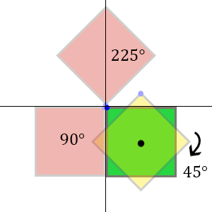
Lets start with the basics behind rotation in 2D. Say you have a nice image you wish to rotate shown here as the green square. If you want to rotate it by 45 degrees, you will want to expect the yellow square here. For some of you this will be perfectly normal, and it should be. However, usually when you rotate an image in your code and look at what happens, we see the red squares appear when rotating 90 or 225 degrees. How does this happen, and more importantly how do we fix this?



Going back to the digital world, we have some other sense of logic. It will all make complete sense in a moment but bear with me. An image is usually represented as a 2 dimensional array of information, starting at [0,0] and ending at [X,Y] with X as width and Y as height of your image. So the least you know about your image is it starts at [0, 0], right? Thats exactly why this ‘bad’ rotation from green to the red squares happens. I marked the top left corner of the image with a blue dot, this is the position [0,0] of your image. As you'll see this blue dot will stay pretty much on the axis I’ve drawn. So, if you would just say to your compiler:
"rotate my image 90 degrees!" Your compiler would just say: "okay, I will rotate it around the origin for you, you have not specified anything so I will assume your origin is centered at [0, 0]!" Hence the result shown in the image above shows up.

So how do we fix this? We want to get the result shown as the yellow square above. To realise this we have to rotate the image around its own axis. Shown in the image is the center of the green square with a black dot. What we want to do here is set the axis for the rotation on this point. So basically you just put a hinge in the center of the square and rotate it around that. Now to represent this in the digital world, lets go back to the origin of your image: [0, 0]. We want this origin to be the center of the green square.



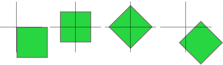
For the complete rotation to work you will have to move the square so that the center of the image is positioned at the axis, shown here in the image above. Once you have done this you can rotate your image freely without consequences. At the end don’t forget to return it to its original position!

This was it for part 1 of this tutorial. In the next part we will continue on doing this correct rotation by using matrices and then applying it on 3D models.

Continue to part 2