Sunday, June 7, 2020

Computing arithmetic gymnastics

Today was a day well spent on programming a bruteforce solution to a simple arithmetic puzzle. The puzzle is something I came up with during a daydream a long time ago. It’s simple arithmetic gymnastics for when you have nothing better to do.

You start off with a 4 digit number, let’s take 1234 as an example. The goal is to create a sum out of the separate digits with any of the four basic mathematical operations: add, subtract, multiply or divide, where the answer to this sum must be exactly zero. You may switch the order of any digit, and add parentheses everywhere.

Correct examples in this case would be:

1 + 2 + 3 + 4 = 10
1 - 2 + 3 - 4 = -2
(1 + 3 - 4) * 2 = 0

Where the last example would satisfy the condition and create a solution in this case.

I found that every number I tried had a solution, and I could not find a number that was not solvable. However the question remained: is every 4 digit number solvable? So today I set out to find the answer.

Programming out the problem

When we calculate a solution to this problem, we often use heuristics to quickly find obvious solutions. The most obvious strategy is that when a number contains a zero, you can just multiply all numbers and end with a zero. Another simple strategy is found when you have two digits that are the same, subtracting the two will create your zero and hence the solution again.

Before arriving at heuristics to speed up computation I wanted to solve this problem the hard way: brute forcing a solution. Since computers can do way more instructions per second than I do solving simple arithmetics, this should be easy to solve for a problem this size. I did not care for performance at first, the simplest solution would do. The language of choice was C# for its ease of use.

The problem at hand is easy to imagine, since we are very used to calculating these numbers daily. It is however harder to program out all possible solutions. The method I used to arrive at a solution was to use some combinatorics.

Part one: calculating all possible number combinations

The first observation I made was that some of the operations were not commutative: subtraction and division produce different results when you swap the digits around. For this reason we would need all permutations of the numbers instead of combinations, since the order in which numbers appear does matter!

Creating a recursive function to generate all possible digit permutations looks as follows:

private static IEnumerable<int[]> CalculatePermutations(IEnumerable<int> list, int length)
{
    if (length == 1)
        return list.Select(t => new [] { t });

    return CalculatePermutations(list, length - 1)
        .SelectMany(x => list.Where(element => !x.Contains(element)), (t1, t2) => t1.Concat(new [] { t2 })
        .ToArray());
}

I create all permutations up to a given length, which is useful if we want to solve the problem with more or less than 4 digits later on. Note that this function is used to create permutations of unique indices and not the numbers themselves. This has two advantages: we can move the computation out of the for loop for every number, and we don’t have to deal with duplicate number permutations.

Part two: all possible operator combinations

Similar to the digits we will have to fill N-1 operators between the digits with any of the arithmetics. However in this case we need permutations with repetitions, as the multiply operator could be used multiple times for example.

We can realize this by creating the same function as previously mentioned with a small change: we don’t filter results that have duplicates:

private static IEnumerable<T[]> CalculatePermutationsWithRepetition<T>(IEnumerable<T> list, int length)
{
    if (length == 1)
        return list.Select(t => new [] { t });

    return CalculatePermutationsWithRepetition(list, length - 1)
        .SelectMany(x => list, (t1, t2) => t1.Concat(new [] { t2 })
        .ToArray());
}

Stringing it all together

Now that we have all possible number and operator permutations we can start adding them together. The sum will be solved from left to right, simply accumulating the result during the process. Note that all numbers will have to be floating point numbers since we involve a division operator that can lead to fractions.

But what about the parentheses? Since we have all possible permutations for every number and for every operator, we generate all possible orders. However this does not include all possible parentheses, it's easy to see that the combination:

1 / (2 + 3 + 4) 

is never included with the possible orders since we only calculate the sum from left to right. I have decided to leave out non-commutative solutions as this would introduce another set of permutations, and thus increasing the already factorial runtime even more.

The findings

I ran the simulation for multiple solution spaces, 1 digit numbers up to 7 digit numbers. For each of these ranges I calculated the amount of numbers that had a solution and converted those to percentages as seen in the graph below.


The 0-10 digit range is easy to explain, one zero equals 10 percent. The two digit realm doubles these numbers, as you have numbers containing zeroes (10, 20, etc) and one other combination of similar digits per each ten numbers (11, 22, etc) adds up to 20 percent. I expected the three digit numbers to be very hard to solve, as it’s quite easy to come up with numbers that can’t be solved. I never thought that it would practically be little more than a coinflip whether or not a random number could be solved!

The four digit range will finally answer my burning question of the ages: 97.3 percent of all numbers in this range had an answer! That explains why I never found a number that could not be solved. Basically one in every 40 four digit numbers you come up with should be impossible to solve, yet I never encountered one thus far.

As I initially expected, if you have more numbers to work with the puzzle should get more probable to have a solution. It probably isn’t easier to solve, but the solution is out there!

While the graph above has a neat explanation for each range, the numbers are a bit incorrect, here’s why: in the range of 10-100 we consider 90 numbers, some of which are double and some of which are not. For example 35 and the other permutation 53 both appear, but this is not the case for 60, since “06” was a single digit number. The graph below shows the percentages if we take this minor difference into account:


Digging deeper

Of course I didn’t stop here. While I was implementing this solution I started out with numbers that were only integers to test. Using only integers, I could not use divisions. I wondered if there were any numbers that only had a solution with one or more divisions.

This resulted in arguably the most interesting result from the whole experiment. The exact count of numbers that only have a solution using one or more divisions in the 4 digit range: 24. As I soon realized this is equal to the amount of permutations of a 4 digit number!

That means there is exactly one number (in a variety of different orders), and that number is 3468. I took the moment to appreciate the beauty here and just calculated numerous ways of solving it.

What is it about that 2.4% of numbers that have no solution? Strikingly similar to the above, 2.4% of 10000 equals 240 numbers. Once more we can see that these are permutations of 10 unique numbers. These are the 10 numbers:

1468
1479
1579
3678
3789
4568
4678
4689
5679
5789

Unfortunately I can’t find some black magic that ties all these numbers together yet, but maybe you can! Be sure to let me know! Below are two data pieces I gathered for all of these numbers: their sum, and the permutation of digits and operators that came the closest to zero.


The final thing I calculated is what would change if the solution was a different number than zero:
Which looks like something close to a skewed normal distribution. Interesting solutions were -24 with just over 50% and 72 with just under 50% of all numbers generating a solution.

Conclusion

Thanks for taking the time to read about this overanalyzed strange number game. I hope you still learned a thing or two from this futile effort to promote my nonsense arithmetics. If you enjoy me getting enthusiastic about absolutely nothing, feel free to bookmark this page.

Wednesday, August 21, 2019

Ryne

I just released a tech demo of Ryne, my game-engine-to-be. You can find more information and media on the Ryne Engine website.

Ryne is an experimental voxel pathtracer. You can try the tech demo yourself to see if it runs on your PC.

In the future I will release the C# scripting side open source. This will allow you to change most of the engine features yourself. You can see an overview of the functionality currently included in that project here


Why “release” it now?

I don’t want to create endless videos about a new technology that you will have to believe is real. Instead I’d like to include as many of you as possible while Ryne is in development. I know Ryne still has flaws and is nowhere near as usable as I want it to be, but I’m still convinced that putting out tech demos like these will bring the point across that we will get there eventually. This will both help me focus on the most important issues, and make everyone aware this is no longer a dream, but we can actually render something right now.

I’m trying to keep a stream of releases going out whenever I feel a new set of features or bug fixes are good to go.

If you’d like to discuss or have more questions, feel free to join the discord server.

Monday, April 23, 2018

Cryptocurrencies in (p)review

And now for something completely different. Recently a new sector of technology caught my attention: cryptocurrencies. Of course, most of you reading this will know about this piece of technology by reading news headlines on the ridiculous price growth of Bitcoin. In this article I will try to create an overview of the whole crypto space.

All over the internet you can find people either praising bitcoin or completely criticizing its existence. Even in the investing world there are "Bitcoin maximalists", people who only invest in Bitcoin and ignore all other cryptocurrencies. My view on Bitcoin is pretty neutral, there are both advantages and disadvantages to the almost 10 year old cryptocurrency. The largest upside is the fact that everyone knows Bitcoin exists, a miracle on its own. The downside is the (already) dated tech: Bitcoin has run into major problems with transaction speed and transaction costs. A solution is already being released: Lightning Network, but it may be too little too late.

Enough about Bitcoin. There is one other topic I have to address before we can have a good discussion about the technology rather than its price: investing. Just like the opinions on Bitcoin, investing in cryptocurrencies is a hot topic, and will probably spike the news again if prices rally up. The question is always "should I invest in cryptocurrencies?". The only answer to this question has to be: decide for yourself. Before you race to Google, be aware that most, if not all, sources of information contain a certain bias. You could for example visit the cryptocurrency subreddit and find a lot of people are positive on certain currencies. On the other hand I found this article from MrMoneyMustache, even though its negative outlook, pretty informative. Either way, this post is not about investing, but rather the technology behind several cryptocurrencies.

I hope to have retained enough readers after the last paragraph, so below a short statement on why cryptocurrencies are still in its infancy:


The reason why I became so interested in cryptocurrencies has nothing to do with the price of a certain cryptocurrency. I got interested because almost all of the projects are completely open-source! This open-source state is such an interesting shift compared to all currently closed source companies. There is even a page that monitors activity on all the GitHub crypto repositories.

Other than the code being free to view for everyone, I was astounded by the creativity of some projects. Some of the interesting projects that I encountered are listed below (hint: this is where you can find my bias)

IOTA: An Internet Of Things solution for the crypto world, using what they call the "Tangle", a technology placed in the category of "Blockchain 3.0". The IOTA team tries to solve the original peer-to-peer transaction problem with a revolutionary but simple method: you as a user of the network will have to verify two other transactions on the network when you enter a new transaction. Their paper is very in depth on safety and even discusses resistance to quantum computing. Interestingly enough I stumbled upon a good friend of mine in both IOTA and NANO: DAG (Directed Acyclic Graphs), which I happen to use for compressing Sparse Voxel Octrees (see other blogposts ;) ).

Storage solutions on the blockchain. A very interesting idea. You can upload files completely anonymous, and nobody in the world is able to take down your file (except if they happen to have the power to cut off all existing nodes). Notable mentions are Oyster Pearl and SIA which are decentralized solutions for storage being launched.

Battling recent changes in the US on Net Neutrality are projects like Substratum and the recently announced Oyster Shell. These projects aim to create a decentralized web, where you can use the internet by connecting through other users instead of central authorities like internet providers. Unfortunately this is only a software solution as the hardware between users can still be controlled by centralized authorities.

Blockchain application platforms like Ethereum and NEO allow for hosting other cryptocurrencies and dapps (decentralized applications) on their network. Ethereum being the second oldest crypto, is currently hosting 1385(!) projects. Cryptolights is an interesting visualization of some transaction speed comparisons for mainstream cryptocurrencies. Even though it is faster than Bitcoin, Ethereum has also hit its limits when a famous app called CryptoKitties was released.

Privacy coins like Monero and Enigma mask public transactions by scrambling a group of transactions together. Enigma even allows for private data inside "secret contracts", which are able to perform the necessary computation without knowing the complete dataset.

There are too many awesome projects to list here, I left out some other interesting projects like to keep this article reasonably short. You can always check CoinMarketCap yourself and find more projects.

So what now?
We have seen the power of blockchain and the positive sides of the crypto world, so we have to conduct a reality check and look at the "dark side of crypto". The most important problem that urgently requires solving is the power consumption. This page shows bitcoins power consumption:


The power consumption at the moment of typing is comparable to all of Switzerland. One single transaction can power about 32 US households for a day. On the other hand, this article compares the current banks and VISA's power consumption versus Bitcoin. It shows a rough estimate of all power consumption by the current banking system worldwide, which is of course more than bitcoin, but banks won't be completely replaced by Bitcoin. There will still be buildings and computers that need to be powered, even though the work on them will probably change.

The problem mainly exists because of the current financial incentive generated by what is called mining in the crypto world (also known as Proof Of Work). Users offer their computational power to compute the solution to a cryptographic problem for the next transaction (where many gamers expressed outrage, for whom graphics cards became an expensive purchase). If only there was another solution readily available for Byzantine fault tolerance.. Luckily some projects already adapted POS (Proof Of Stake) methodology, where users can stake to be a decision node on the network. Examples like Ethereum's Sharding and NEO's DBFT give me hope for a more eco-friendly solution.

A second problem is found when looking at the current state of the crypto world. There are currently around 1600 currencies in existense, of which most projects will completely fail, or are complete scams. This seems to be comparable to the dot-com bubble, where many internet startups went bankrupt when the market collapsed.

Finally I see the statement "crypto makes money laundering way too easy" a lot. Guess when a similar statement also appeared: when everyone was speculating about the invention called "the internet". I can't say it isn't a problem, but removing all privacy from the crypto space isn't the solution either.

But you promised a discussion
Now that I have overloaded you with information, let's dive even deeper. Why does this technology exist? Why did Satoshi Nakamoto (creator of Blockchain and Bitcoin) publish this paper anonymously, and dissapeared? There are a lot of unanswered questions in this space, and I can't wait to see the documentary on the crypto space a decade from now.

Would you say that this technology is predetermined? This article lists a good reason why such an evolution was a logical step (using technology to lower the economic cost). After all, the technology was already predicted in 1999.

Put yourself in Satoshi Nakamoto's place for a moment. Would you go public? I think he has enough reason to stay anonymous. Going public might make him responsible for oppressing the government or banking systems. On the upside, you have a lot of Bitcoin..

How about measuring what such a network is actually worth: this article builds on a previous article of the Network Value to Transactions (NVT) ratio. The NVT ratio is used as the "crypto PE ratio" in order to compare crypto "stocks" in a similar fashion as stocks. The NVT ratio is based on Metcalfe's law, a measure of the network in terms of its users. While it's reasonably accurate, it would be interesting to see a ratio that also measures transactions that happen off-chain, for example exchange transactions.


Whether or not any of the currently existing currencies survive, I do think the technology will trigger a global shift in how we deal with data. Blockchain technology (and all of its successors) have excellent usecases for dealing with personal data. We could use the technology to make the data immutable (meaning no information tampering is possibe) and more private. Maybe the dystopian fiction of having a small chip underneath your fingernails containing your private key will even become reality..

Finally, my hopes for the future are to become less dependent on central organizations managing all the world's currency and make a shift towards a decentralized solution, while we keep dreaming about a distributed network for efficiency. With this overview article I hope to have sparked your interest in this network of "trust based on distrust".

Did I miss something important, or do you want to discuss? Let me know in the comments.

Sources:
https://en.wikipedia.org/wiki/Lightning_Network
https://trends.google.com/trends/explore?q=bitcoin
https://blockchain.info/nl/charts/avg-confirmation-time
https://bitinfocharts.com/comparison/bitcoin-transactionfees.html
https://www.reddit.com/r/CryptoCurrency/
https://www.mrmoneymustache.com/2018/01/02/why-bitcoin-is-stupid/
https://coincheckup.com/analysis/github
https://www.iota.org/
https://nano.org/en
https://oysterprotocol.com/
https://sia.tech/
https://substratum.net/
https://www.ethereum.org/
https://neo.org/
https://getmonero.org/
https://enigma.co/
https://www.coindesk.com/cat-fight-ethereum-users-clash-cryptokitties-congestion/
https://coinmarketcap.com/
https://hackernoon.com/the-bitcoin-vs-visa-electricity-consumption-fallacy-8cf194987a50
https://en.wikipedia.org/wiki/Proof-of-work_system
https://en.wikipedia.org/wiki/Byzantine_fault_tolerance
https://en.wikipedia.org/wiki/Proof-of-stake
https://github.com/ethereum/wiki/wiki/Sharding-FAQ
https://steemit.com/neo/@basiccrypto/neo-s-consensus-protocol-how-delegated-byzantine-fault-tolerance-works
https://steemit.com/blockchain/@skane/a-vision-of-a-hivemind
https://medium.com/cryptolab/https-medium-com-kalichkin-rethinking-nvt-ratio-2cf810df0ab0
https://en.wikipedia.org/wiki/Metcalfe%27s_law
https://medium.com/@bbc4468/centralized-vs-decentralized-vs-distributed-41d92d463868

Thursday, July 6, 2017

Automated marshalling of managed- to unmanaged structures

An art that I wouldn't even wish upon my greatest enemies to figure out.

I recently started a new project in a language very familiar to me: C#, a managed language. This means that all the memory management is done for you, which is both a blessing and a curse. For this project, I happened to struggle over the "curse part" of automatic memory management.

The problem I encountered is as follows: when you have two structures that are identical in terms of their members, their respective sizes can (and often will) differ in managed languages compared to unmanaged languages. For example, I have the following structure in C# and C++ respectively:

// C#
[StructLayout(LayoutKind.Sequential)]
struct DebugComponent
{
    public float4 Float4;
    public float Float;
}

// C++
struct CPP_DebugComponent
{
    float4 Float4;
    float Float;
};

The size of the structure can be found in C# by using Marshal.SizeOf() (or sizeof() in unsafe code) and reports that the structure is 20 bytes in size, which is correct. Note that I already applied the StructLayout to Sequential, as this will create a layout similar to unmanaged code.

The size of the same structure in C++ using sizeof() reports that the structure is 32 bytes. This is also correct, because the float4 type here is aligned to 16 bytes, meaning the structure will receive another 12 bytes of padding at the end, to make sure it aligns with 16 bytes.

Unfortunately trying to use this structure in a tool such as ManagedCuda, the CUDA kernel struct will use the C++ version, and when you call the kernel from your C# code you will have to use the other version. This creates a mismatch in memory layout, resulting in very weird artifacts after running the kernel, or even crashing because you're writing to unallocated memory in this case.

The "simple" solution I found is to manually expand the C# structure by using the StructLayout.Size attribute to extend the structure to 32 bytes instead of 20. After asking my question on StackOverflow, I didn't solve the problem to create these structures automatically without counting the sizes of every individual type in the structure itself.

So I had to switch up my solution a little bit. I created a project which contains the raw C# structures that I want to use, along with all their functionality like loading and serialization. I then created another C# project for the automated code generation. Using this project we can load our Structures as a dll, from which we can derive all the structures and what types they contain in text templates:
  • Structures: project that contains raw structures that will be used on the GPU
  • Tools: my general purpose project that will generate GPU versions of the structs defined in Structures.
In order to make this conversion as secure as possible I don't want to manually check every time I create a new structure if the GPU version has the same alignment and size. So I created two more projects:
  • AlignedStructsWrapper: A C++/CLI project that combines managed and unmanaged code
  • Tests: a unit test project
Using the CLI project, we can load both our versions of the structure: the managed C# version and the unmanaged C++ version. We can now measure the difference in their sizes:

public ref struct WrapperGpuDebugComponent
{
public:
 int SizeDiff()
 {
  int managedSize = sizeof(Tools::Content::Generated::DebugComponent);
  int nativeSize = sizeof(CUDA::CPP_DebugComponent);
  return managedSize - nativeSize;
 }
};

In the unit test project we load our CLI from reference and we can create a simple unit test that calls the SizeDiff function and checks if the difference is indeed 0:

[TestMethod]
public void CheckStructureSizes()
{
 WrapperGpuDebugComponent debugcomponent = new WrapperGpuDebugComponent();
 Assert.AreEqual(debugcomponent.SizeDiff(), 0);
}

Of course I also generated the CLI structures and the unit test functions automatically for every structure so I only have to recompile the projects and have everything tested.

Sunday, May 14, 2017

CUDA in Visual Studio 2017

Edit: CUDA 9.0 RC is released. This version shows full Visual Studio 2017 support.

Note: this article only shows how to compile Visual Studio 2015 CUDA projects in Visual Studio 2017. For actual VS2017 support we will have to wait for a new CUDA release.

I previously wrote a small article on CUDA support for VS2015, to support CUDA compilation of older projects. Following the same principle we can 'hack' CUDA compilation support in VS2017. 

What you need
  • CUDA installation with visual studio integration for VS. I used CUDA 8.0 and VS2015 respectively.
  • VS2017 (any edition)
Copying the required files
  • To allow CUDA compilation we have to copy a few files. Find the CUDA 8.0 setting files in the VS2015 buildcustomizations directory:
C:\Program Files (x86)\MSBuild\Microsoft.Cpp\v4.0\V140\BuildCustomizations
Note: If you use a different VS version, you have to change the 'V140' accordingly (V120 for VS2013 for example).
  • Copy the following files: CUDA 8.0.props, CUDA 8.0.targets, CUDA 8.0.xml, and Nvda.Build.CudaTasks.v8.0.dll
  • Find the VS2017 buildcustomizations directory:
C:\Program Files (x86)\Microsoft Visual Studio\2017\Community\Common7\IDE\VC\VCTargets\BuildCustomizations
Note: I used the VS2017 Community edition. If you have another edition, change 'Community' in the path accordingly.

  • Paste the CUDA files here.

That's it
You can now load and compile your VS2015 CUDA projects in VS2017. When you first open your project in VS2017, make sure to not upgrade your project to VS2017, otherwise this won't work. 

Friday, April 28, 2017

IniGenerator

I wrote a simple C# code interface for ini files. There are already great NuGet packages for ini file IO parsing and writing, but not a lot of packages that automatically generate a code layer. For this project I based my solution on the ini parser to do the file IO.

My package only provides a small overlay to create a C# class which handles all the file IO behind the scenes. Using the text-templates, we define both the ini file and create a C# class. An example file I used to create my configuration:

<#@ include file="$(ProjectDir)IniTemplate.tt" #>
<#
    // All properties in the ini file
    // Name, default value and category
    CreateProperty("Width", 1280, "Video");
    CreateProperty("Height", 720, "Video");
    CreateProperty("Fullscreen", false, "Video");

    // Generate the code layer
    GenerateIniClass();
#>

Which will create a C# class with the same name as your text-template. The ini file will either be created the first time you use this class, or the old values will be read from the existing file.

Usually there is no backwards compatibility with older versions of the ini file. If you add new properties, all values in the ini file will be reset to their defaults. I avoid these scenarios using the beautiful functionality to merge two ini files from the ini parser. I can simply add the new properties to the old ini file without changing their values.

Finally, an example of the above template used in code:

// Use the namespace where you placed the template
using IniGenerator.Content.Generated;

// Name of ini file
var config = new Config();
// Can be used directly in code without parsing
var size = new Size(config.Width, config.Height);
var fullscreen = config.Fullscreen;

You can view the source code on GitHub, or download the package from NuGet.

If you have any feedback, leave a comment or post an issue on the GitHub project.

Saturday, April 22, 2017

Master Thesis

Update: You can download the full thesis here.

Level-of-Detail Independent Voxel-Based Surface Approximations was the subject of my master thesis. I wrote a small dissemination that explains the basics of my thesis on this page.


This image shows the final result of my thesis work. The models above are voxel models with 4096 (2^12) voxels in every axis. If they were all filled, I would have to store 4096^3 = 68719476736 voxels in total. There has been a lot of research into compressing the huge amount of data this requires, I mentioned some examples on the thesis page.

Using a Sparse Voxel Octree (SVO) storing scalar field values, the six models above can be stored in 12GB of memory total. Using my multiresolution method we can store visually comparable models in only 2GB of memory total.

Here is a small video showing the current state of the voxel path tracer:


Thursday, October 27, 2016

Master thesis current state

For my master thesis, I've been working on a project for some time now. In this post I'll share a few debug screenshots of the current state of the project.


The project can load triangle meshes of (almost) any format, and convert them to large resolution sparse voxel octrees (SVO). In the picture above, you can see the voxelized Lucy model, which is about 500MB in triangle format.

Converted to an SVO, storing only which voxels are on or off, we can store data for up to 4096^3 voxels in only ~40MB. That's a boolean for ~68 billion voxels. But since we only store voxels that are on, this number changes drastically, thus we are able to compress this pretty well.

If you want to store more data for every voxel, the amount of memory is going to skyrocket. In the example above, I store a scalar field for every voxel (that's 8 floating point numbers per voxel). All that data nets nearly 870MB for the highest resolution.

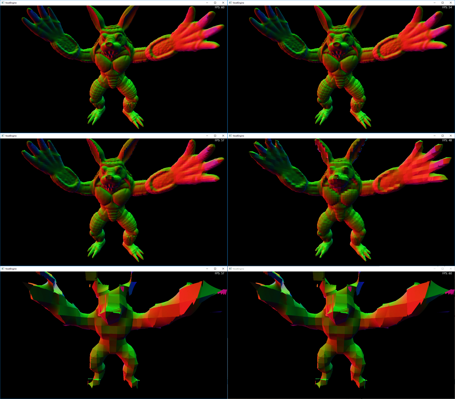
I was able to convert and draw a model up to 8192^3 resolution, including all simplifications of a dragon model:


Where you can see that the voxel resolution is even larger than the millions of triangles stored in the model.

For my master thesis I will be working on creating level of detail simplifications. The screenshots below show some results of a linear approximation calculated for a group of voxels:


The first model at 512^3 resolution, and the second at 2048^3.

These images are rendered using raymarching to find the intersection point of a ray and a scalar field. I wrote the raytracer in CUDA, which allows for an interactive framerate even with gigantic data sets by using parallelization on the GPU.

Finally, some more renders:


Wednesday, July 20, 2016

The next step in Entity Component Systems

Let's talk game engines. For a current project, I'm writing a game engine completely from scratch. Before I started I wrote down some key functionalities the engine should be able to handle. After writing that down, the proces of creating the engine boils down to optimizing the functionality in terms of performance and memory requirements.

Before we dive into engine compositions, let's look at two big AAA game engines used to create games which are used by a large number of developers today.

Unreal Engine 4 is mostly known because of the impressive graphics that can be created within a few mouseclicks. The engine is open source, and is an all-round engine that supports nearly everything you can think of when creating a game. Below you will find some amazing pictures rendered using Unreal Engine 4.


Complete album here.

Unity is an all-round game engine designed to ease the development process by working with C# as its core language. Unity is a lot more oriented towards an entity component system than Unreal Engine 4.


These engines took years to develop, and can practically support any use case. For my engine I'm looking to only support a very narrow subset of these use cases.

The thing both engines have in common is that they are both entity component systems, which is what the remainder of this post is all about.

Engine compositions
Mainly, there are two compositions for game engines. The first one is Object Oriented Programming (OOP), and the second type is an Entity Component System (ECS). There are already a lot of resources available to learn about both. I compiled a small list of examples, and will revisit the topic briefly.

[1] Understanding Component-Entity-Systems by Boreal Games
Shows a clear and concise introduction to OOP vs ECS systems.
[2] Implementation of a component-based entity system in modern C++ by Vittoreo Romeo for CPPCon
Explains the ECS system in depth and shows an implementation in C++
[3] Evolve your Hierarchy by Mick West
Experience from a programmer changing from OOP to an ECS system. Explains cache optimizations

Object Oriented Programming
The main reason to use OOP for games, was that the concept is easy to grasp. You create a hierarchy for all objects, and code reuse is introduced by polymorphism. In the diagram below you can see an example of OOP used in a game engine.

Image from [1]
It's clear to see that the EvilTree can't fit in the hierarchy, because it would require inheritance from both static and dynamic entities. While this is possible in some languages, it can lead to difficulties known as the diamond problem.

Entity Component System
The entity component system is designed to solve the problem stated above. The structure above would look as follows in an ECS:

Image from [1]
Where you can see that all the objects are derived from different components. The components can be reused for any object, this makes it easy to add new entities.

The next step for Entity Component Systems
Now that we are up to speed with game engine compositions, let's look at the path forward.

Data Oriented Design (DOD)
This paradigm is the design principle behind the ECS system. The basic principle is instead of looking at code, look at data. This concept is derived from the fact that most applications are memory bound instead of processing power.

The main point for DOD in game engines focusses on using the ECS in a way that avoids cache misses. To illustrate this, we look at the table below.

Image from [3]
In this ECS from [3], we can see on the left all the entities in the game, and in the table all of the components they exist of. When viewed from a higher scale, the only thing we changed is instead of looking at the diagram from left to right, we now look at it from top to bottom. So in our code we define our components as a list of Position components, Movement components, and so on.

For every entity we add, we simply add one of each component to all component arrays. This is why there are holes in the diagram.

All the way at the top of this article, I said that the engine is a balance between performance and memory. We can now clearly see why this is the case: this layout consumes a lot of memory to increase the performance. The "Script only" object creates 5 empty components which will never be used.

The three principles
We can define three points to weigh all our engine needs.
  1. Cache efficiency
  2. Memory efficiency
  3. Parallel efficiency

Now we have to define how to determine the efficiency of all of these points.
  1. Measuring cache efficiency is tricky at best, and this is very dependent on optimization. So instead of a ratio, we define the following: An engine becomes more efficient if we require fewer arrays available at the same time, and the smaller the size of a single item in the array the better
  2. The ratio for memory efficiency is defined as the total used components divided by the total created components.
  3. We can determine the parallel efficiency by looking at the percentage of work that can be executed in parallel. For a complete calculation of the speedup, we can look at Amdahl's law.

ECS revisited
Now that we have the three principles, we can discuss the efficiency of the ECS system. If we assume that we are using the ECS from [3]:
  1. We can see that this would lead to a good cache efficiency, but not the best: A physics component can't operate without a position component, this means we need multiple arrays simultaneously when updating entities. But the big advantage here is that all the arrays are separated, and can be queried individually per component.
  2. The memory efficiency is bad. The ratio for this particular example is already 19/30 = 63%. That means that 37% of our memory is just thrown away for the sake of efficiency.
  3. The parallel efficiency leads to a tricky scenario: how can you execute ECS in parallel? In this particular case, we pretty much can't. The physics system updates the position component, and only after that, we can render the component using the new position.

    In order to process everything in parallel, we'd have to look from left to right (per object) again, and processing the objects in parallel would require ALL data available in caches, which in turn would lead to a lot of cache misses.. 

In conclusion, we can say that we traded off space for time. We require more memory, but less processing time due to cache efficiency to process all our objects.

As for parallel efficiency, from a DOD composition such as this, we can run some tasks in parallel. If we look at the implementation from [2], every entity has a signature:

Image from [2]

In this case, the signature tells us that we require AI and Enemy components. In the implementation, we have systems that update all entities containing specific signatures. To create a simple parallel processing ECS, we can simply say that every set of systems that don't have any component in common can execute at the same time.

In our example, with a physics system and rendering system, this would not work, since they both rely on a position component.

A solution presented in Vittorio Romeo's presentation is to store all the components in one mega-array:

Image from [2]
While this could be the solution, I very much disliked the amount of work required to implement this, and keep up with all the overhead of adding and removing components.

Setting up the engine
In my engine I opted for an ideal solution, within the constraints of C++ (static types, known at compile time). With the power of C++ 11, we can reach a lot using variadic templates, and I built a lot of my implementation with it.

I based my system on the implementation of [2]. I use signatures to define a set of components, and I also define systems by providing a signature. But instead of storing components separately in one array per component type, I took a step back in 'engine progression'. I define one array for every possible signature.

If you read that carefully, you should already be thinking, that would require a lot of arrays! If we define up to 64 different components, and generate one array for every possible signature, we would have 1.8446744073e+19 arrays. Possibly requiring more memory than the complete application that we're building.

So instead of creating one array for all possible signatures, let's create one array for every signature used. The tricky part is finding all possible signatures at compile time. And we can't do that in C++, since we have no such library as reflection from C#, where we could query all that.

Text templates
We will use C# to create our signatures before the C++ compile time, so we know all the types at compile time. For this we will use something commonly used in web development: text templates. If it's your first time working with these in visual studio, I recommend the syntax highlight plugin.

So in text templates, we can write code that writes code, quite nifty. A small example that generates a list of all our components:

<#@ template debug="false" hostspecific="false" language="C#" #>
<#@ assembly name="$(TargetDir)CodeGeneratorFunctions.dll" #>
<#@ import namespace = "CodeGeneratorFunctions" #>
<#@ output extension=".h" #>
// This file was automatically generated
#pragma once
<#
 string[] components = Generator.GetComponents();
 foreach(string component in components)
 {
  WriteLine("#include \"Components\\" + component + ".h\"");
 }
#>

Where I define a function "GetComponents()" in a DLL CodeGeneratorFunctions, to search all our files for component signatures. I was pleasantly surprised with the runtime, as I thought it would take years to search all those files, but it actually took less than a couple of seconds.

Similar to this example, I wrote text templates for all signatures and systems.

The engine
Back to engine talk, now that we have our component composition, let's determine how efficient this engine could be in theory.

  1. Cache efficiency. At first glance, the cache efficiency would suffer in comparison with the original ECS from [3], but it's hard to tell. We have a larger single item size in the array, but we only require one array simultaneously. Below I explain a small optimization that reduces the individual item size. 
  2. Our memory efficiency is great. Since we can basically store only the necessary components for every object, we waste 0% of memory, with a little overhead of creating a lot of arrays in larger systems. 
  3. The parallel efficiency is similar to the ordinary ECS. We can only execute systems in parallel when they contain unique component sets. 
So in theory, we got an advantage in terms of memory. But we are still questioning if the cache efficiency changed. Looking back at the mega-array structure, we can see that we improved a little, we can store our velocity and position together in one array, so we don't have to acces two separate arrays and have cache misses. 

Optimizations
The main disadvantage of this structure is when you use larger objects. If we have an object storing a lot of components, the item size of the array is going to be large. And a large item size means cache misses. We can make our engine more cache friendly by using hot/cold data separation

As example, we consider objects storing data for physics (position, velocity) and rendering (huge models of 300MB). Loading only two of these objects, is a guaranteed cache miss, since the two objects are 300MB apart in the memory lane. The solution is to store a reference to the model, rather than storing it completely, and only call the model when it's required for rendering. This way we can update the physics without cache misses (a pointer is only 8 bytes). 

The hot/cold data separation separates hot data (used multiple times) versus cold data (used sparsely). If you want to read more, I suggest reading the article on gameprogrammingpatterns about this topic


To improve up on the parallel execution of the system, we can schedule all the work of one system in parallel. Since one system will be handling multiple arrays of objects, the first option is to execute all of these in parallel, and the second option is to execute all of the items in one array in parallel. Since the arrays have different lengths, the first option would be a bad choice (one thread would take very long, while the others would be waiting). Thus linearly processing all arrays, and execute all items inside that array is the best option. Further optimizations can be done by using SIMD instructions, but that is outside the scope for this article. 


Future work
I'd like to see if I can increase parallel efficiency by introducing tech from Naughty Dog's engine. They have a great presentation about it available online. Instead of introducing parallel execution per system, I'd like to see if we can create a set of instructions per signature and create a fiber to execute that.

When I'm done creating the engine (which is never, because it's a game engine) I will compile some benchmarks compared to a 'normal' ECS implementation. I also hope to release some source code from this engine.

Sources
[1] Understanding Component-Entity-Systems by Boreal Games
[2] Implementation of a component-based entity system in modern C++ by Vittoreo Romeo for CPPCon
[3] Evolve your Hierarchy by Mick West
[4] What is data oriented design StackOverflow
[5] Introduction to data oriented design DICE
[6] Gameprogrammingpatterns: Data Locality
[7] Parallelizing the Naughty Dog engine using fibers

Thursday, February 25, 2016

CUDA in Visual Studio 2015

Update September 2016: CUDA 8.0 is available, Visual studio update 3 is supported.
Update June 2016: CUDA 8.0 RC is available. Visual studio 2015 is supported, but update 2 is not yet included.

In this small post I will explain how you can use CUDA 7.5 in Visual Studio 2015. I don't claim to have full support for VS2015, merely using the VS2015 editor and compiling a VS2013 project. You will still need to have Visual Studio 2013 installed, with the CUDA toolkit extension.

On a separate note: Nsight does have support for VS2015, so no hacks required there!

What you need:

  • Any C++ project using CUDA.
  • CUDA 7.5 toolkit with VS2013 support installed (I only tested it with 7.5, but I can imagine other versions working as well)

In the project properties, make sure the project compiles for "v120", which is VS2013. 

To actually load the project in VS2015 having support for compiling CUDA code, we have to copy some files. Visual Studio uses targets to include several extensions for loading project files. We simply have to copy the VS2013 support to the VS2015 folder:

The CUDA 7.5 extension files for VS2013 are located in:
C:\Program Files (x86)\MSBuild\Microsoft.Cpp\v4.0\V120\BuildCustomizations

Find CUDA 7.5.props, CUDA 7.5.targets and CUDA 7.5.xml

If you simply copy them to the same folder for VS2015:
C:\Program Files (x86)\MSBuild\Microsoft.Cpp\v4.0\V140\BuildCustomizations

You can now load these projects in VS2015. 


My raytracer running from VS2015 using Nsight. 

Monday, December 21, 2015

Real-time Raytracing part 4

In all of the previous posts, I've talked about optimizing ray tracing. I've mentioned path tracing, but never spoke of path tracing specific optimizations. This post will be a small survey of implementations and research about path tracing optimizations.

Foundations

Path tracing is great for simulating global illumination by tracing rays, and of course, these rays have to follow "realistic paths". As observed a long time ago (1760) by Johann Lambert, intensity of light from an ideal diffuse surface is directly proportional to the cosine of the angle $\theta$ between the direction of the incident light and the surface normal. This is called Lambert's cosine law in optics.

In path tracing, we mainly use the cosine law to calculate the contribution of light from the next ray. When tracing from a diffuse surface, the direction of the next ray is usually calculated by generating a random direction in the hemisphere of the surface. When tracing from a mirror, you can imagine there is only one direction on the hemisphere that is correct: the perfect reflection. Metal-like surfaces contain both elements, called glossy reflections. This image shows what I'm talking about in 2D:


If you would order them by calculation cost for the path tracing algorithm, the reflection would be the easiest, there is only one solution, one ray to calculate. The glossy one is harder to calculate, since you have to accumulate rays with different weights, but still simpler to fully calculate than the diffuse option. Besides these simple examples, materials can contain many functions to bend incoming rays. The collection of these functions describe the Bidirectional Reflectance Distribution Function (BRDF). Which in turn, you can even extend to allow for rays extending through the surface with a Bidirectional Scattering Distribution Function (BSDF).

Cosine weighted sampling
The intensity of light from an ideal diffuse surface is directly proportional to the cosine of the angle $\theta$ between the direction of the incident light and the surface normal.
This leads to an interesting optimization: cosine weighted sampling. Since the incoming and outgoing light is measured by a cosine, the outgoing rays nearly parallel to the surface don't add any (useful) information to the final solution. I could write this whole post about this optimization, but that would be a waste of time, since there are already many good examples out there. This post from Rory Driscoll shows results as well as the maths behind it.

This image shows the cosine weighted sampling on the top and the uniform sampling on the bottom. This was taken from the pathtracing blog
Sampling optimization

As mentioned above, when you've found a ray-triangle collision, the direction of the new ray is usually 'bruteforce' calculated by taking a random direction on the hemisphere. For diffuse surfaces, this is no problem, since every outgoing direction weights the same. If you would apply the same to perfectly reflecting surfaces, chances are you will most likely never find the correct outgoing ray.

By knowing the material properties you can determine how to sample the outgoing ray. This sampling strategy can be a very easy optimization if you're willing to end up with an approximation. If you look at the 3 examples from the image above: one variable for the degree of reflectiveness can produce these examples.

The problems with this reflectiveness variable for path tracing are the weights shown in the glossy example. Solving the Monte Carlo problem of path tracing requires a probability distribution function (PDF) over these samples. The outer rays in the glossy examples are shown smaller, because they affect the outcome less than the rays from the perfect reflection.

This optimization is as simple or as hard as you want to make it. The simpler you keep the sampling, the more approximate your solution is going to be. The best solution would be to sample your chosen BRDF. The cosine weighted sampling is shown to be perfect for diffuse only materials (diffuse materials have perfect lambertian reflectance). I found a sampling method for the Cook-Torrance BRDF in this paper: Microfacet Models for Refraction through Rough Surfaces.

Direct and indirect lighting

Direct lighting is easy to calculate. This is shown in almost all released 3D games out there. Simply calculating a dot product of the surface normal and light direction would result in perfect lambertian shading.

In path tracing we can apply an optimization to allow for direct light sampling. It's called next event estimation. This is where the math and statistics get nasty. To allow for direct light sampling, we have to apply a different probability distribution function. We have to sample the light and divide the contribution of direct light by the area of the light:
Area sampling. Image taken from [2]

Whereas the indirect illumination should be sampled by the original method using hemispheres. With one exception, all of the rays hitting the light should be discarded (since the light gets sampled by the other PDF from above).
Hemisphere sampling without direct light sampling (dashed lines). Image taken from [2]
These examples show only sampling of a single light, which is easy to maintain. Imagine a scene with thousands of lights and one sun. If you apply the same theory of the two PDFs from above, you would end up sampling more inefficient than the brute force sampling. The solution is rather simple, we add weights to each light. But these have to be based on different criteria: only adding weights based on distance could influence the effects of the sun (large distance, huge brightness) versus normal lights (small distance, small brightness). Other small optimizations could be added based on needs: you don't have to continually sample the sun during night time and so on. If you like to know the mathematics and details behind these two PDFs, I suggest you read the presentations from the references below.

Multiple importance sampling

In larger applications, thousands of material types and BRDFs are going to be used. Having a different sampling strategy for each of them is going to be time consuming and frankly undo-able. We already have two different PDFs to sample all of these materials, the direct and indirect sampling. The problem that arises from all of this shown in images:

These are the two sampling methods shown from above, the BSDF sampling is the hemisphere indirect sampling and the light source sampling is the direct sampling using the area of the light. The problem is the glossy reflection on the four plates. You can see that indirect sampling works if the light is large enough to have some collisions with rays, and the direct light source sampling works fine for small area lights.

Multiple Importance Sampling is a technique that can combine different sampling techniques to find a low variance estimate of the integral. By combining both sampling methods we can get the following result:
Images taken from [4]

Bidirectional path tracing

This leads us to more recent techniques in path tracing, namely bidirectional path tracing. This technique is based on the inverse of path tracing, instead of finding the light by tracing rays from the camera, find the camera by tracing from the light. These are the shooting rays, and the original camera rays the gathering rays. The bidirectional part indicates that these two types of rays can be combined.

This technique wasn't meant for real time path tracing applications which require responsiveness. Since for every gathering ray you shoot, the amount of calculation is doubled by also tracing shooting rays. This nearly doubles the time per frame, and thus decreases responsiveness. While you lose responsiveness, this algorithm increases the convergence rate for path tracing a lot, so in the end it's worth it.

As extension to bidirectional path tracing, there is an algorithm called Metropolis light transport. This algorithm allows finding more difficult light paths by extending existing paths. An example: A shooting and gathering ray have been found by the bidirectional raytracing method. Every bounce in these rays is recorded as a node. The metropolis light transport can add extra nodes on these rays to modify the existing ray to a new one. These nodes are placed in areas with high gradients. You can find more on this technique in this paper: Metropolis Light Transport.

Another extension I found, but have not fully explored is: Light Transport Simulation with Vertex Connection and Merging. The basic idea is to reuse existing paths by connecting vertices. This can increase the amount of generated paths per pixel:

Vertex merging: reusing paths to increase paths per pixel. Image taken from [6]
There is an opensource implementation of VCM called smallVCM. This implementation also contains multiple importance sampling and normal bidirectional path tracing.

Further reading

Most recent techniques include gradient domain tracing. It first originated from metropolis light transport in: Gradient-domain Metropolis Light Transport. The paper on Gradient Domain Bidirectional Path Tracing applies this to a bidirectional path tracer, and Gradient-Domain Path Tracing applies the same principle for normal path tracers. The path tracer also contains source code. You can see the path tracing algorithm is converging faster already with only one sample per pixel:

Showing the difference between Gradient domain path tracer (G-PT) and normal path tracer (PT). Image taken from [9].
Other blog posts:

http://blog.hvidtfeldts.net/index.php/2015/01/path-tracing-3d-fractals/
Path tracing 3D fractals. Also explains cosine weighted sampling, importance sampling, next event estimation, and image based lighting. Implementation in GLSL.

http://raytracey.blogspot.com
Everything about ray tracing, and is currently working on a GPU path tracer.

https://www.reddit.com/r/pathtracing/
https://www.reddit.com/r/raytracing/
Community for path- and ray tracing.

References

Presentations

[1] http://cg.informatik.uni-freiburg.de/course_notes/graphics2_09_pathTracing.pdf
[2] http://www.cs.dartmouth.edu/~cs77/slides/18_PathTracing.pdf

Papers

[3] Walter, Bruce, et al. "Microfacet models for refraction through rough surfaces."Proceedings of the 18th Eurographics conference on Rendering Techniques. Eurographics Association, 2007.
[4] Veach, Eric. Robust monte carlo methods for light transport simulation. Diss. Stanford University, 1997.
[5] Veach, Eric, and Leonidas J. Guibas. "Metropolis light transport." Proceedings of the 24th annual conference on Computer graphics and interactive techniques. ACM Press/Addison-Wesley Publishing Co., 1997.
[6] Georgiev, Iliyan, et al. "Light transport simulation with vertex connection and merging." ACM Trans. Graph. 31.6 (2012): 192.
[7] Lehtinen, Jaakko, et al. "Gradient-domain metropolis light transport." ACM Transactions on Graphics (TOG) 32.4 (2013): 95.
[8] Manzi, Marco, et al. "Gradient-Domain Bidirectional Path Tracing." (2015).
[9] Kettunen, Markus, et al. "Gradient-domain path tracing." ACM Transactions on Graphics (TOG) 34.4 (2015): 123.


Saturday, December 5, 2015

Real-time Raytracing part 3.1

In part 3, I've shown some examples on how to tune algorithms on the GPU. Here I would like to address how we can apply those rules to optimize path tracing. As usual, I will show code samples for CUDA, but this doesn't mean it can't be applied on any other graphics programming language.

Fortunately for us, there is an opensource framework for optimized GPU based ray traversal. The framework is from the research paper Understanding the Efficiency of Ray Traversal on GPUs. In 2012 they added Kepler and Fermi Addendum, which added some changes to the framework to optimize traversal for those architectures. In this post I will be looking at the version for the kepler architecture. The framework is quite heavy on magic numbers and hard to read code. In this post I'm going to dissect some of the more important parts and how they improve performance.

Data structures

The first thing to notice is what kind of spatial data structure they are using. From the name of the class: "SplitBVHBuilder" you can already see that the builder is based on this paper. It comes down to a simple binned BVH builder, including triangle splits to optimize traversal. For more information on BVH techniques, you can read part 2 of this series.

More important for this post is how you store this BVH on the GPU and access it without creating any memory latency. If we look at the ray traversal, the following code shows how the nodes are read from memory:

    const float4 n0xy = tex1Dfetch(t_nodesA, nodeAddr + 0); // (c0.lo.x, c0.hi.x, c0.lo.y, c0.hi.y)
    const float4 n1xy = tex1Dfetch(t_nodesA, nodeAddr + 1); // (c1.lo.x, c1.hi.x, c1.lo.y, c1.hi.y)
    const float4 nz   = tex1Dfetch(t_nodesA, nodeAddr + 2); // (c0.lo.z, c0.hi.z, c1.lo.z, c1.hi.z)
            float4 tmp  = tex1Dfetch(t_nodesA, nodeAddr + 3); // child_index0, child_index1
            int2  cnodes= *(int2*)&tmp;

Recalling from part 3, I showed you a similar statement for memory alignment using the fact that arrays in global memory didn't have data fragmentation. Reading memory from a texture using this principle is more natural, because textures ensure no data fragmentation. As seen in the comments above, the information gathered contains two BVH bounding boxes and two child indices. Storing the data this way ensures you have four 128 bit reads and one 64 bit read, since the last two values are unused.

The other data structure I would like to point out is the way they store triangles. The nodeaddr variable can store either positive or negative values. The positive indicate an index in the BVH and negative values store indices to the triangle array. The actual index is found by using the bit negate function ($\sim$) on the index. From this address they fetch the triangle using similar code as above:

    // Tris in TEX (good to fetch as a single batch)
    const float4 v00 = tex1Dfetch(t_trisA, triAddr + 0);
    const float4 v11 = tex1Dfetch(t_trisA, triAddr + 1);
    const float4 v22 = tex1Dfetch(t_trisA, triAddr + 2);

In which you can store the data required for a ray-triangle test and execute it. The thing to note is: BVHs can store more than one triangle per node, especially SBVHs. In order to store this efficiently in one array, they inserted breaks in the array. The code for checking all triangles:

for (int triAddr = ~leafAddr;; triAddr += 3)
{
 // Read triangle data (see above)

    // End marker (negative zero) => all triangles processed.
    if (__float_as_int(v00.x) == 0x80000000)
        break;

 // Ray-triangle intersection (see part 1)
}

The for loop determines the triangle address and loops endlessly increasing the triangle address. If the first address contains a stop value (they chose for negative zero, but any distinguished value will do), stop the for loop. Simple as that, the array can now contain more than one triangle per node.

Traversal algorithm

The traversal algorithm is as follows: beginning this algorithm assumes the ray hit the BVH containing the model we wish to test for. If it didn't, it's not that bad, after two ray-box intersections the algorithm stops.

  • Starting from the first node address, we read the first two child bounding boxes using the code above
  • Using the optimized intersection test for the GPU from the paper, we test ray-box intersections.
  • If the ray intersects one of them, we change the node address and continue the algorithm. 
  • If we intersect both children, store one of the children on the stack and continue traversing the other.
  • If we intersect none, pull a child index from the stack. If the stack is empty, stop the algorithm.
While this algorithm is pretty easy to implement, optimizing it for the GPU is quite a hassle. In order to minimize divergence, they thought of two neat tricks to alter this algorithm. The first trick is persistent threads. This concept originated from the following thought: A warp will execute until all threads inside it are done processing. In a path tracer like ours this can lead to horrific situations: 31 threads waiting for just the one to be done tracing.

The idea to combat this is quite simple: if there are less than X threads active, fetch new work for the idle threads. Using older graphics hardware, the implementation would take some time for all threads to communicate their status using shuffle functions. Since kepler architecture there are some warp voting functions introduced. From the CUDA toolkit:
__all(predicate):
Evaluate predicate for all active threads of the warp and return non-zero if and only if predicate evaluates to non-zero for all of them.
__any(predicate):
Evaluate predicate for all active threads of the warp and return non-zero if and only if predicate evaluates to non-zero for any of them.
__ballot(predicate):
Evaluate predicate for all active threads of the warp and return an integer whose Nth bit is set if and only if predicate evaluates to non-zero for the Nth thread of the warp and the Nth thread is active.

Which comes in very useful for this task. The code that remains to execute this test:
if( __popc(__ballot(true)) < DYNAMIC_FETCH_THRESHOLD )
                break;
Where __popc is a population count, counting the number of bits equal to 1 from the provided value.

The other trick in the algorithm to minimize divergence is part of triangle checking. It comes down to timing: when to check for triangles. In theory, the threads in the warp could be divergent: one thread checking ray-triangle intersections and the others traversing the BVH. While this is not completely preventable, we could help the algorithm postpone checking triangles until all threads have at least one triangle to check.

By creating an array (or in this case a variable) to store a triangle address, we can continue traversing the BVH until other threads have also found a triangle. The code in the source uses a direct compiled statement to check this, since it wouldn't be compiled in an optimal way. The code that you would need to check if all threads have a triangle is simple:
    if(!__any(leafAddr >= 0))
        break;
Where leafAddr indicates a triangle address. The statement simply checks if there is a thread for which the address is larger than or equal to 0. If there are none, it means all threads have found a triangle to check and we can stop traversing the BVH.


I hope to have cleared up some of the magic parts of the source code. Of course, if you have any more questions about it, feel free to post them below.